GETPIVOTDATA Function in Excel – Complete Guide (Basic to Advanced)
If you work with PivotTables in Excel, you must have noticed that when you try to reference a cell inside a PivotTable, Excel automatically inserts the GETPIVOTDATA formula instead of a simple cell reference.
Many beginners find this function confusing, but in reality, it’s one of the most powerful tools in Excel for extracting specific data from a PivotTable accurately.
In this blog, we’ll explain:
What is GETPIVOTDATA
Its syntax & arguments
How to enable/disable it
Practical examples
Advanced tips to use it effectively
The GETPIVOTDATA function is used to extract specific data from a PivotTable report based on given field names and item names.
It ensures you get accurate data even if the PivotTable layout changes.
Category: Lookup & Reference Function
Introduced in: Excel 2007 and later
Works with: All PivotTables
| Argument | Description |
|---|---|
| data_field | The name of the data field to extract (in quotes). |
| pivot_table | Any cell reference inside the PivotTable. |
| field1, item1 | (Optional) Field name and item name to fetch specific data. |
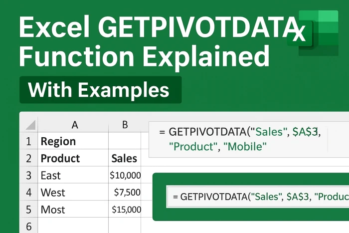
You have a PivotTable showing Product Sales by Region. You want to extract total sales for “Mobile” from the PivotTable.
Formula:
Explanation:
"Sales" → Data field name
$A$3 → Any cell inside the PivotTable
"Product","Mobile" → Extracts sales for “Mobile”
If your PivotTable has Product, Region, and Month, and you want to fetch sales for Laptop in North region for January, use:
This gives exact values, regardless of the PivotTable structure.
By default, Excel automatically inserts GETPIVOTDATA when referencing PivotTable cells.
Go to PivotTable Analyze → Options
Click the Drop-down Arrow under Options
Toggle “Generate GETPIVOTDATA” ON/OFF
✅ Always fetches accurate data
✅ Works even if PivotTable layout changes
✅ Supports multiple criteria
✅ Great for dynamic dashboards
| Problem | Reason | Solution |
|---|---|---|
Returns #REF! |
Incorrect data field name | Use correct field names from PivotTable |
| Wrong results | Field names not matching | Use exact spelling & case |
| Too complex | Multiple fields used | Use helper cells for clarity |
Use named ranges for PivotTables to avoid cell reference errors.
Combine GETPIVOTDATA with IFERROR to handle missing data.
Use it with SUM, AVERAGE, and dynamic dashboards.
Q1. Why does Excel automatically insert GETPIVOTDATA?
Because Excel assumes you want accurate data from a PivotTable instead of a simple cell reference.
Q2. How do I stop Excel from using GETPIVOTDATA?
Disable Generate GETPIVOTDATA under PivotTable Options.
Q3. Can I use GETPIVOTDATA with dynamic reports?
Yes, you can link it with drop-downs, slicers, and dashboards.
The GETPIVOTDATA function in Excel is an essential tool for anyone working with PivotTables. It helps you extract specific, accurate data and is extremely useful for dynamic reports and dashboards.
If you want to master Excel and learn advanced formulas, practice GETPIVOTDATA along with other functions like VLOOKUP, INDEX, and MATCH.